Webpage and simulations written by Moshe Mishali and Yilun Chen.

Conventional sub-Nyquist sampling methods for analog signals exploit prior information about the spectral support. A more challenging problem is spectrum-blind sub-Nyquist sampling of multiband signals. For example, cognitive radio receivers face with this kind of problem whenever sensing the RF spectrum at their surroundings. The modulated wideband converter (MWC) is the first system for sub-Nyquist sampling, which can be realized with existing devices and handle wideband analog signals. This enables, for example, realizing a carrier-unaware cognitive radio receiver, as further described in this paper. This page describes the MWC system and provides two simulation packages for signal recovery from samples obtained by the MWC (see below on the differences between these packages). The recovery performance is measured in Monte-Carlo setup, namely by using the MWC for sampling and reconstruction a large number of randomly-drawn multiband inputs, and reporting the average recovery accuracy over these test inputs. These packages were used to create the figures in the research papers. A simplified version of these simulations, which is described in this page,  simulates a single realization of a multiband input via a convenient graphical user interface (GUI). In addition to signal reconstruction, this page demonstrates carrier frequencies estimation and information bits decoding of concurrent narrowband digital transmissions.

Signal model. The Fourier transform of wideband signals often occupies only a small portion of a wide spectrum, with unknown frequency support. For example: in wideband communication, the receiver sees the sum of several radio-frequency transmissions. Each signal is modulated around an unknown and different carrier frequency.

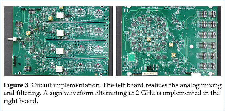
The system. With an efficient hardware implementation and low computational load on the supporting digital processing, the modulated wideband converter (MWC) can blindly sample multiband analog signals at a low sub-Nyquist rate. The MWC first multiplies the analog signal by a bank of periodic waveforms. Then the product is lowpass filtered and sampled uniformly at a low rate. The waveform period and the uniform rate can be made as low as the expected width of each band, which is orders of magnitude smaller than the Nyquist rate. Reconstruction relies on recent ideas developed in the context of analog compressed sensing, and is comprised of a digital step which recovers the spectral support. The MWC enables baseband processing, namely generating a low rate sequence corresponding to any information band of interest from the given samples, without going through the high Nyquist rate. In the broader context of Nyquist sampling, the MWC scheme has the potential to break through the bandwidth barrier of state-of-the-art analog conversion technologies such as interleaved converters.

• M. Mishali and Y. C. Eldar, "From Theory to Practice: Sub-Nyquist Sampling of Sparse Wideband Analog Signals", IEEE Journal of Selected Topics on Signal Processing, vol. 4, no. 2, pp. 375-391, April 2010.
• M. Mishali, Y. C. Eldar, O. Dounaevsky and E. Shoshan, "Xampling: Analog to Digital at Sub-Nyquist Rates", IET Circuits, Devices & Systems, vol. 5, no. 1, pp. 8–20, Jan. 2011.
• M. Mishali and Y. C. Eldar, "Blind Multi-Band Signal Reconstruction: Compressed Sensing for Analog Signals", IEEE Trans. on Signal Processing, vol. 57, no. 3, pp. 993-1009, March 2009.
• M. Mishali and Y. C. Eldar, "Reduce and Boost: Recovering Arbitrary Sets of Jointly Sparse Vectors", IEEE Trans. on Signal Processing, vol. 56, no. 10, pp. 4692-4702, October 2008.
• M. Mishali and Y. C. Eldar, "Expected RIP: Conditioning of The Modulated Wideband Converter", Information theory workshop (ITW), pp. 343-347, October 2009.

• Matlab package that simulates sampling by the analog system. The MWC consists of an RF front-end whose intermediate nodes are non-bandlimited signals. In this setting, computing the samples that would have been obtained by the hardware becomes a tricky task. This package sets the MWC parameters properly and also uses a dense time-grid in order to ensure sufficient approximation in computing the analog samples. The simulations in this paper were generated by this package.

• A simulation package of the MWC of a digital counterpart of the RF front-end. In this setting, the input signal is a vector of samples which is assumed to have a multiband support in the DFT domain (which in general is not true for a set of samples of an analog multiband input). Although this demonstration is not simulating the analog system, it has a prominent advantage -- the runtime is considerable shorter, since there is no need to approximate the input on a dense time grid. It can help to ease the understanding of the system and the simulation setup, which is similar to the previous package, up to a few different line codes (see the comments in the body of the CTF block below).

The modulated wideband converter (MWC) is comprised of two stages: sampling and reconstruction.

In the sampling stage, the input signal enters a bank of multiple channels simultaneously. In each channel, the input signal is multiplied by a mixing function. The mixing function is designed to be a periodic random bit-sequence. Its purpose is to spread the spectrum such that a portion of energy from each band appears in the baseband. After mixing, the signal spectrum is first truncated by a lowpass filter and then sampled at a low rate corresponding to the lowpass cutoff, yielding multiple channels of low-rate digital samples.

In the reconstruction stage, the low-rate digital samples enter the continuous-to-finite (CTF) block for spectrum support estimation. Once the unknown support of the spectrum is determined, the active bands of the input signal are reconstructed by digital processing and mature DAC technology.

The signal of interest is a multiband signal consisting 3 pairs of bands (total N = 6 bands, as depicted in Fig. 1). Each band is of width B = 50MHz and of energy 1, 2, and 3. Ttime offsets are specifed by Taui, to better visualize the results. The Nyquist rate of the multiband signal is supposed to be as high as 10GHz.

SNR = 10;                       % Input SNR
N = 6;                          % Number of bands (when counting  a band and its conjugate version separately)
B = 50e6;                       % Maximal width of each band
fnyq = 10e9;                    % Nyquist rate
Ei = [1 2 3];                   % Energy of the i'th band
Tnyq = 1/fnyq;
R = 1;                          % The length of the signal is R*(K+K0)*L

K = 91;
K0 = 10;                        % R*K0*L is reserved for padding zeros
L = 195;
TimeResolution = Tnyq/R;
TimeWin = [0  L*R*K-1 L*R*(K+K0)-1]*TimeResolution; % Time interval in which signal is observed
Taui = [0.7 0.4 0.3]*max(TimeWin);     % Time offest of the i'th band

fprintf(1,'---------------------------------------------------------------------------------------------\n');
fprintf(1,'Signal model\n');
fprintf(1,'   N= %d, B=%3.2f MHz, fnyq = %3.2f GHz\n', N, B/1e6, fnyq/1e9);

We use 50 low-rate sampling channels to sample the 10GHz multiband signal. The sampling rate for each channel is fs = 10GHz/195 = 51.3MHz. Therefore, the actual sampling rate is 51.3MHz*50 = 2.56GHz.

ChannelNum = 50;                            % Number of channels
L = 195;                                    % Aliasing rate
M = 195;
fp = fnyq/L;
fs = fp;                                    % Sampling rate at each channel, use fs=qfp, with odd q
m = ChannelNum;                             % Number of channels

% sign alternating  mixing
SignPatterns = randsrc(m,M);                % Draw a random +-1 for mixing sequences

% calucations
Tp = 1/fp;
Ts = 1/fs;
L0 = floor(M/2);
L = 2*L0+1;

fprintf(1,'---------------------------------------------------------------------------------------------\n');
fprintf(1,'Sampling parameters\n');
fprintf(1,'   fp = %3.2f MHz, m=%d, M=%d\n',fp/1e6,m,M);
fprintf(1,'   L0 = %d, L=%d, Tp=%3.2f uSec, Ts=%3.2f uSec\n', L0, L, Tp/1e-6, Ts/1e-6);

Now we generate the input signal using the following codes. The carriers of the signal are randomly assigned.

t_axis = TimeWin(1)  : TimeResolution : TimeWin(end);     % Time axis
t_axis_sig  = TimeWin(1)  : TimeResolution : TimeWin(2);

fprintf(1,'---------------------------------------------------------------------------------------------\n');
fprintf(1,'Continuous representation\n');
fprintf(1,'   Time  window = [%3.2f , %3.2f) uSec\n',TimeWin(1)/1e-6, TimeWin(2)/1e-6 );
fprintf(1,'   Time resolution = %3.2f nSec, grid length = %d\n', TimeResolution/1e-9, length(t_axis));
fprintf(1,'---------------------------------------------------------------------------------------------\n');
fprintf(1,'Generating signal\n');
% Signal Generation

x = zeros(size(t_axis_sig));
fi = rand(1,N/2)*(fnyq/2-2*B) + B;      % Draw random carrier within [0, fnyq/2]
for n=1:(N/2)
    x = x+sqrt(Ei(n)) * sqrt(B)*sinc(B*(t_axis_sig-Taui(n))) .* cos(2*pi*fi(n)*(t_axis_sig-Taui(n)));
end
han_win = hann(length(x))';             % Add window
x = x.*han_win;
x = [x, zeros(1,R*K0*L)];               % Zero padding

% Calculate original support set

Sorig = [];
% explain:  we take the starting edges: fi-B/2  and divide by fp. minus
% 0.5 to shift half fp towards zero. then M0+1 is to move 0 = M0+1.
Starts = ceil((fi-B/2)/fp-0.5+L0+1);
Ends = ceil((fi+B/2)/fp-0.5+L0+1);
for i=1:(N/2)
    Sorig = union (Sorig,  Starts(i):Ends(i));
end
% Now add the negative frequencies
Sorig = union(Sorig, L+1-Sorig);
Sorig = sort(Sorig);

---------------------------------------------------------------------------------------------
Continuous representation
   Time  window = [0.00 , 1.77) uSec
   Time resolution = 0.10 nSec, grid length = 19695
---------------------------------------------------------------------------------------------
Generating signal

We run the following commands in MATLAB to see the spectrum of the signal.

>> figure, plot(linspace(-5,5,length(x)),abs(fftshift(fft(x)))),grid on 
>> title('Spectrum of x'), xlabel('Frequency (GHz)'), ylabel('Magnitude')

The indices of active bands are:

>> Sorig

Sorig=

11 12 58 59 64 65 131 132 137 138 184 185

The white Gaussian noise is genereated such that its spectrum is in [-fnyq/2, fnyq/2].

noise_nyq = randn(1,(K+K0)*L);              % Generate white Gaussian nosie within [-fnyq/2,fnyq/2]
noise = interpft(noise_nyq, R*(K+K0)*L);    % Interpolate into a finer grid (the same length as the signal)

% Calculate energies
NoiseEnergy = norm(noise)^2;
SignalEnergy = norm(x)^2;
CurrentSNR = SignalEnergy/NoiseEnergy;

Now we mix the input signal and noise with random periodical functions.

fprintf(1,'Mixing\n');

MixedSigSequences = zeros(m,length(t_axis));
for channel=1:m
    MixedSigSequences(channel,:) = MixSignal(x,t_axis,SignPatterns(channel,:),Tp);
end

MixedNoiseSequences = zeros(m,length(t_axis));
for channel=1:m
    MixedNoiseSequences(channel,:) = MixSignal(noise,t_axis,SignPatterns(channel,:),Tp);
end

The random mixing function aliases energies from each bands into the baseband. This is the key step that enables the following baseband operation without losing information.

>> figure,plot(linspace(-5,5,length(x)),abs(fftshift(fft(MixedSigSequences(1,:))))), grid on
>> title('Spectrum of a mixed signal'), xlabel('Frequency (GHz)'), ylabel('Magnitude')

For each channel, we filter the mixed channel with an ideal low pass filter. Then we downsample the high-rate input sequences (19695 samples for each channel) into low-rate ones (101 samples for each channel).

fprintf(1,'Filtering and decimation (=sampling)\n');
% ideal pass filter
temp = zeros(1,K+K0);
temp(1) = 1;
lpf_z = interpft(temp,length(t_axis))/R/L; % impulse response of the low pass filter

SignalSampleSequences = zeros(m,K+K0);
NoiseSampleSequences = zeros(m,K+K0);
fprintf(1,'    Channel ');
decfactor = L*R;
for channel = 1:m
    fprintf(1,'.');  if ( (mod(channel,5)==0) || (channel==m)) fprintf(1,'%d',channel); end

    SignalSequence =  MixedSigSequences(channel,:);
    NoiseSequence   =  MixedNoiseSequences(channel,:);
    DigitalSignalSamples(channel, :) = FilterDecimate(SignalSequence,decfactor,lpf_z);
    DigitalNoiseSamples(channel, :) = FilterDecimate(NoiseSequence,decfactor,lpf_z);
end
Digital_time_axis = downsample(t_axis,decfactor);
DigitalLength = length(Digital_time_axis);

fprintf(1,'\n---------------------------------------------------------------------------------------------\n');
fprintf(1,'Sampling summary\n');
fprintf(1,'   %d channels, each gives %d samples\n',m,DigitalLength);

Filtering and decimation (=sampling)
    Channel .....5.....10.....15.....20.....25.....30.....35.....40.....45.....50
---------------------------------------------------------------------------------------------
Sampling summary
   50 channels, each gives 101 samples

Next, we use CTF block to recover the support of active bands. The following results indicate that we successfully recover the support.

fprintf(1,'---------------------------------------------------------------------------------------------\n');
fprintf(1,'Entering CTF block\n');

% define matrices for fs=fp
S = SignPatterns;
theta = exp(-j*2*pi/L);
F = theta.^([0:L-1]'*[-L0:L0]);
np = 1:L0;
nn = (-L0):1:-1;
% This is for digital input only. Note that when R -> infinity,
% D then coincides with that of the paper
dn = [   (1-theta.^nn)./(1-theta.^(nn/R))/(L*R)      1/L    (1-theta.^np)./(1-theta.^(np/R))/(L*R)];
D = diag(dn);
A = S*F*D;
A = conj(A);

SNR_val = 10^(SNR/10);          % not dB

% combine signal and noise
DigitalSamples = DigitalSignalSamples + DigitalNoiseSamples*sqrt(CurrentSNR/SNR_val);

% Frame construction
Q = DigitalSamples* DigitalSamples';
% decompose Q to find frame V
NumDomEigVals= FindNonZeroValues(eig(Q),5e-8);
[V,d] = eig_r(Q,min(NumDomEigVals,2*N));
v = V*diag(sqrt(d));
% N iterations at most, since we force symmetry in the support...
[u, RecSupp] = RunOMP_Unnormalized(v, A, N, 0, 0.01, true);
RecSuppSorted = sort(unique(RecSupp));
% Decide on success
if (is_contained(Sorig,RecSuppSorted)  && (rank(A(:,RecSuppSorted)) == length(RecSuppSorted)))
    Success= 1;
    fprintf('Successful support recovery\n');

else
    Success = 0;
    fprintf('Failed support recovery\n');
end

---------------------------------------------------------------------------------------------
Entering CTF block
Successful support recovery

Once we determine the support, we can easily reconstruct each signal band by a direct pseudoinverse operation. The signal bands are then modulated to their corresponding carrier frequencies.
All the band signals are then modulated to their corresponding carrier frequencies.

A_S = A(:,RecSuppSorted);
hat_zn = pinv(A_S)*DigitalSamples;  % inverting A_S
hat_zt = zeros(size(hat_zn,1),length(x));
for ii = 1:size(hat_zt,1)                     % interpolate (by sinc)
    hat_zt(ii,:) = interpft(hat_zn(ii,:),L*R*length(hat_zn(ii,:)));
end

x_rec = zeros(1,length(x));
for ii = 1:size(hat_zt,1)                     % modulate each band to their corresponding carriers

    x_rec = x_rec+hat_zt(ii,:).*exp(j*2*pi*(RecSuppSorted(ii)-L0-1)*fp.*t_axis);
end
x_rec = real(x_rec);					      % Reconstructed signal
sig = x + noise*sqrt(CurrentSNR/SNR_val);     % Original noised signal

We finally plot all the results here.

figure,
plot(t_axis,x,'r'), axis([t_axis(1) t_axis(end) 1.1*min(x) 1.1*max(x) ])
title('Original signal'), xlabel('t')
grid on
figure,plot(t_axis,sig,'r'), axis([t_axis(1) t_axis(end) 1.1*min(x) 1.1*max(x) ])
title('Original noised signal'), xlabel('t')
grid on

figure, plot(t_axis,x_rec), axis([t_axis(1) t_axis(end) 1.1*min(x) 1.1*max(x) ]),
grid on,
title('Reconstructed signal'), xlabel('t')

The output SNR is

 >> 20*log10(norm(x)/norm(x-x_rec))

ans = 
 14.9204

Therefore, compared to the conventional Nyquist sampling , the SNR gain is 14.9204 - 10 = 4.9204 (dB).

Note that the simulation above is for a noisy input signal. If the signal is noiseless (this can be implemented by assigning a sufficiently large value to the parameter SNR), then by re-doing the simulation, the pure reconstruction error is calculated to be about 1e-6, which is almost perfect reconstruction.

Software & Hardware:   SoftwareHardwareDemo movies