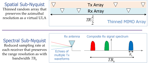
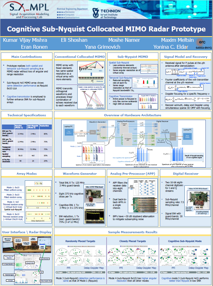
In this demonstration, the radar prototype is designed on the principles of a sub-Nyquist collocated multiple-input multiple-output (MIMO) radar. The setup allows sampling in both spatial and spectral domains at rates much lower than dictated by the Nyquist sampling theorem. Spatial sub-Nyquist allows use of less antenna elements in the array without degrading the angular resolution whereas spectral sub-Nyquist processing uses fewer time samples while maintaining the range resolution (see Figure 1). Our prototype realizes an X-band MIMO radar that can be configured to have a maximum of 8 transmit and 10 receive antenna elements. We use frequency division multiplexing (FDM) to achieve the orthogonality of MIMO waveforms and apply the Xampling framework for signal recovery. The prototype also implements a cognitive transmission scheme where each transmit waveform is restricted to those pre-determined subbands of the full signal bandwidth that the receiver samples and processes. Real-time experiments show reasonable recovery performance while operating as a 4×5 thinned random array wherein the combined spatial and spectral sampling factor reduction is 87.5% of that of a filled 8 × 10 array. This prototype is developed at the Technion and was first demonstrated at IEEE Radar Conference (RadarCon) at Philadelphia in May 2016.

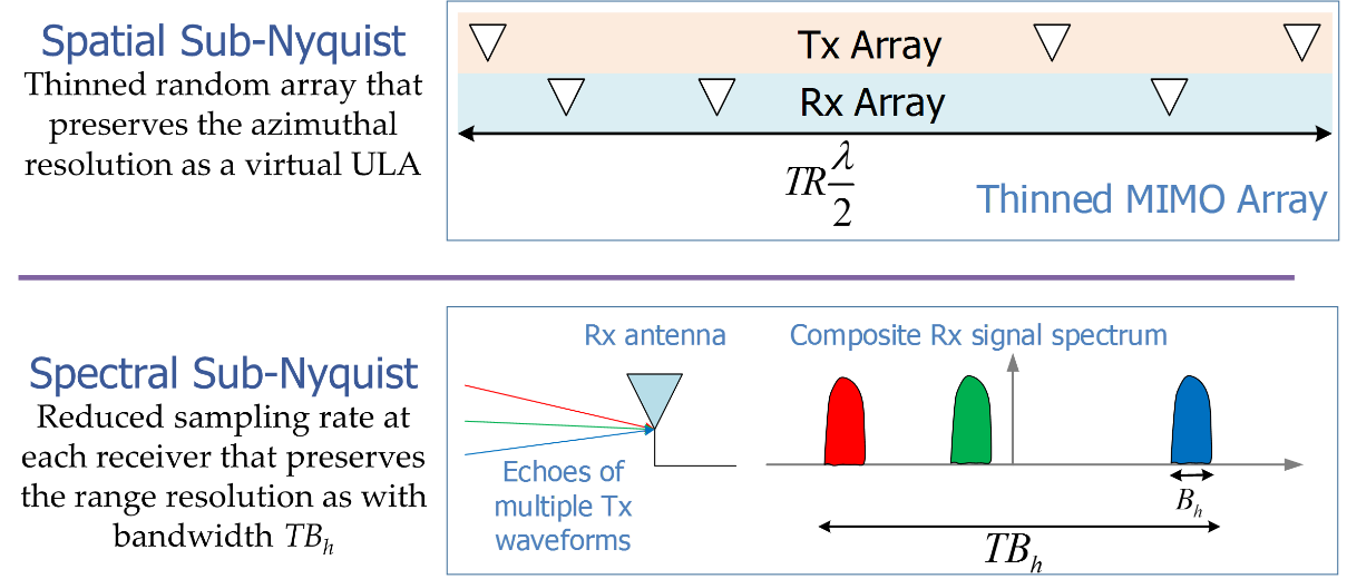
Figure 1. Sub-Nyquist collocated MIMO radar in space and time

Our implementation of the MIMO radar architecture has a maximum of 8 transmit (Tx) and 10 receive (Rx) antenna elements. The spatial and spectral sampling aspects of sub-Nyquist MIMO that we intend to demonstrate manifest only in the receiver processing. Therefore, our radar prototype does not physically radiate the transmit waveforms from an antenna and receive data from actual targets in real-time. Instead, multiple transmit waveforms are pre-computed externally at baseband, their echoes from simulated targets are recorded and the complex samples (in-phase I and quadrature-phase Q pairs) are stored in an on-board memory of a custom-designed waveform generator board. The prototype then processes these pre-recorded signals in real-time.

Similarly, we omit the implementation of the up-conversion to RF carrier frequency in the transmitter and the corresponding down-conversion in the receiver from this prototype. We would assume that the physical array aperture and simulated target response correspond to an X-band (fc = 10 GHz) radar. The choice of radar frequency band also affects the clutter response that we intend to consider in a uture extension of this prototype.

A conventional 8x10 MIMO radar receiver would require simultaneous hardware processing of 80 (or 160 I/Q) data streams. Since a separate sub-Nyquist receiver for each of these 80 channels is expensive, we implement the eight channel analog processing chain for only one receive antenna element and serialize the received signals of all 10 elements through this chain. This approach allows the prototype to implement a number of receivers greater than 10 as the eight-channel hardware only limits the number of transmitters.

For each channel, a single low-rate ADC can subsample this narrow-band signal as long as the subbands are coset bands so that they don’t aliase after sampling. This implementation needs only eight low-rate ADCs, one per channel. Another advantage of this approach is flexibility of the prototype in selecting the Xampling slices. Unlike our sub-Nyquist radar prototype, the number and spectral locations of slices are not permanently fixed, and they can be changed (within the constraints of aliasing due to subsampling).

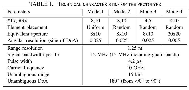
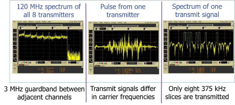
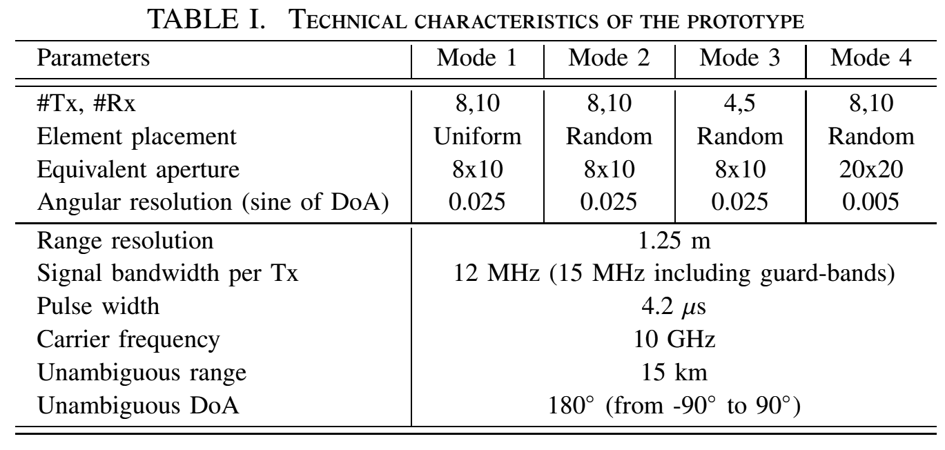
The prototype can be configured to operate in various array configurations or modes. When operating at its maximum strength of 8 Tx and 10 Rx elements, it can be programmed as either a ULA (Mode 1) or a random array (Mode 2), each with the equivalent aperture of an 8 × 10 virtual array, i.e., 1.2 m. For the same aperture, the system can be operated as a thinned 4 × 5 array (Mode 3). In this configuration fewer receivers are serialized and the channels corresponding to the removed transmit elements are not processed by the digital receiver. Mode 3, hence, demonstrates the spatial sub-Nyquist sampling. Finally, the prototype can also function as a 8x10 thinned array (Mode 4) which can be viewed as a spatial sub-Nyquist version of a 20x20 virtual array with aperture of 6 m. Figure 2 shows exact details of element locations for all four modes. Table I summarizes the technical parameters of the prototype for all four array configurations. As mentioned before, this system employs FDM-based signal orthogonality with each transmit signal hm(t) chosen to be approximately flat in spectrum, over the extent of 12 MHz (one-sided band). Each of the transmit waveforms is separated from its nearest neighbor by a 3 MHz guard-band.

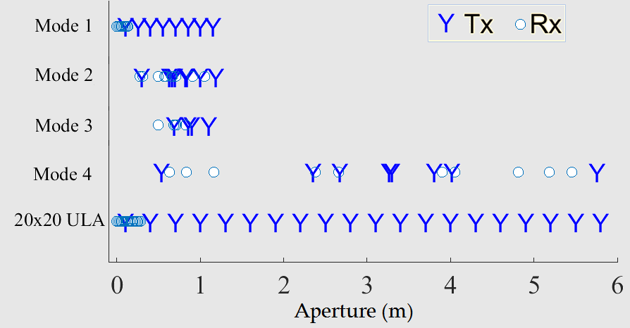
Figure 2. Tx and Rx element locations for the hardware prototype modes over a 6 m antenna aperture.
Mode 4’s virtual array equivalent is the 20 × 20 ULA.

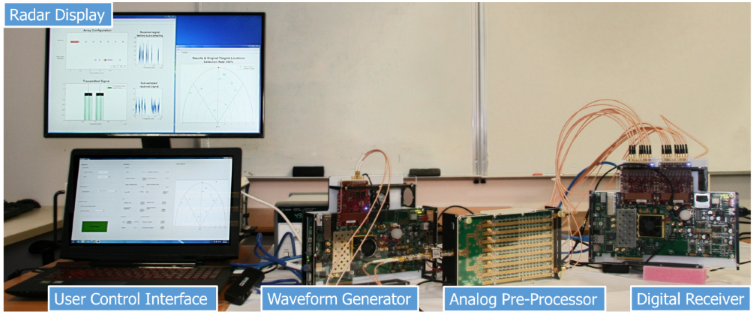
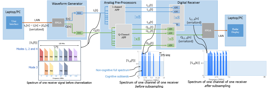
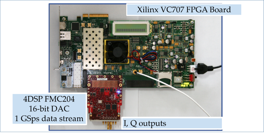
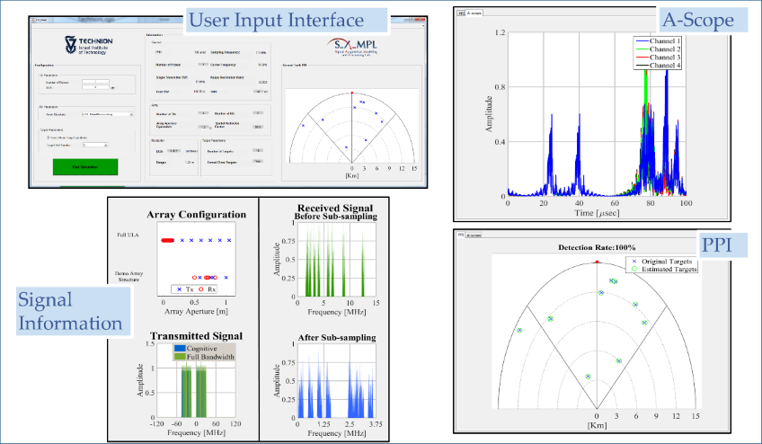
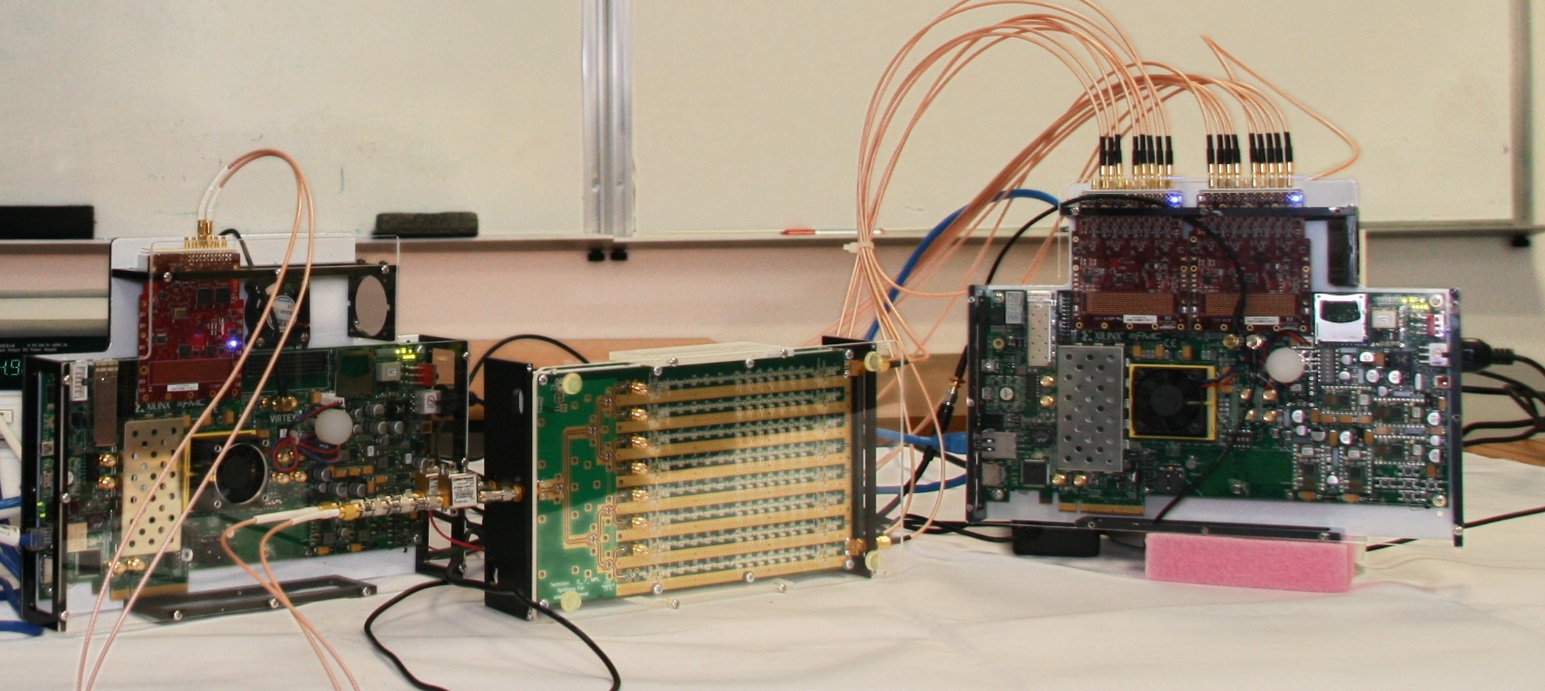
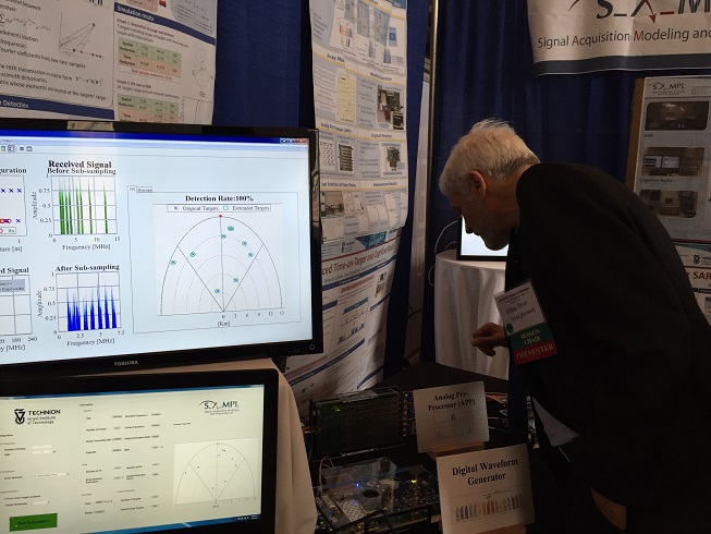
The following Figure 3 shows the sub-Nyquist MIMO prototype, user interface and radar display. Figure 4 shows a simplified block diagram that depicts the signal flow. The user selects the prototype mode from the control interface and passes the control triggers to the transmit waveform generator card (Figure 5), where an FPGA device reads out the pre-stored received waveform from an on-board memory. Two separate digital-to-analog converters (DACs) - one each for I and Q samples - convert the resulting signal to baseband analog domain (Figure 6). The transmit waveform generator is off-the-shelf Xilinx VC707 evaluation board that is custom fit with a 4DSP FMC204 16-bit DAC card. Each of the I and Q analog signals are then passed on to their respective analog pre-processor cards

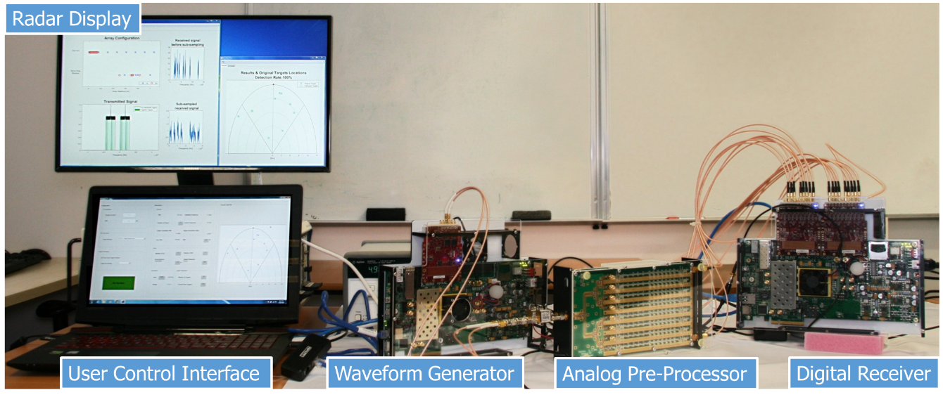
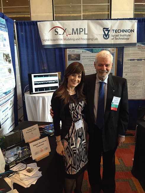
Figure 3. Sub-Nyquist MIMO prototype and user interface.

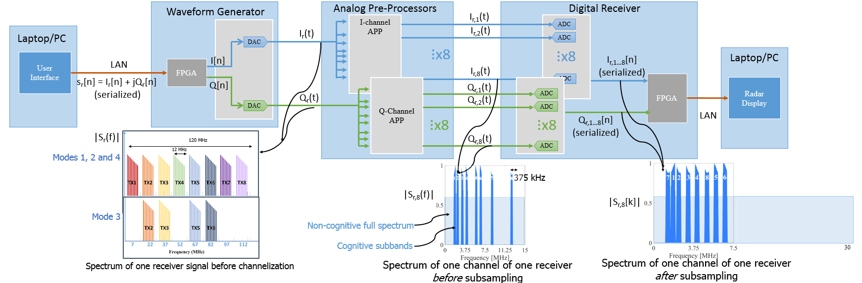
Figure 4. Simplified block diagram of cognitive and sub-Nyquist MIMO prototype. The subscript r represents received signal samples for rth receiver.
Wherever applicable, the second subscript corresponds to a particular transmitter. The square brackets (parentheses) are used for digital (analog) signals.

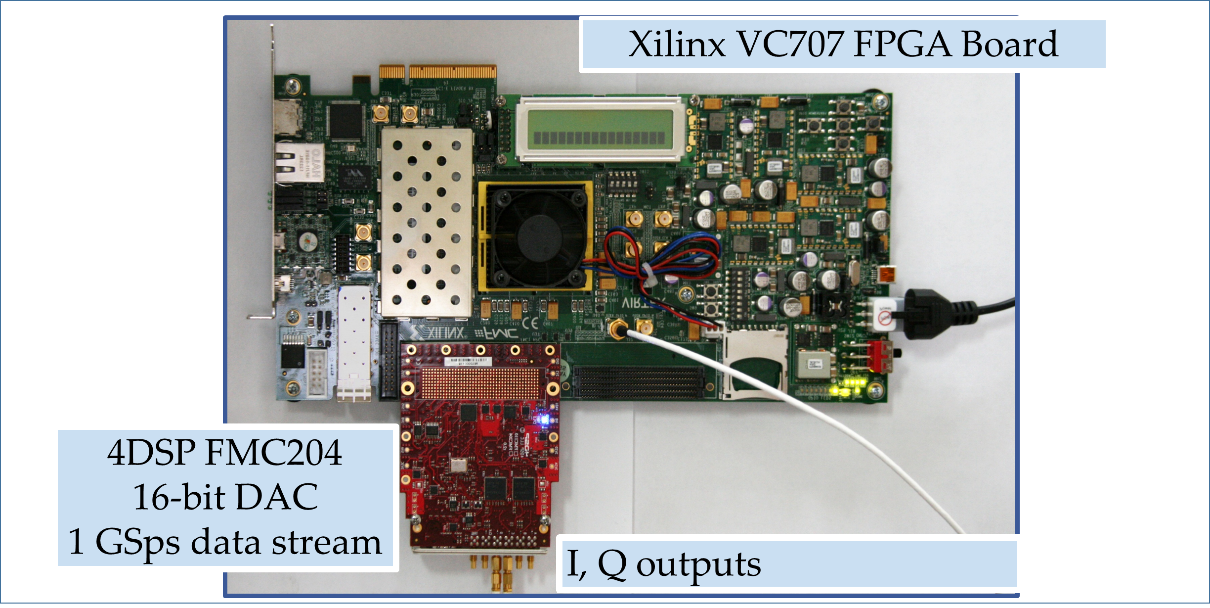
Figure 5. FPGA-based digital waveform generator.

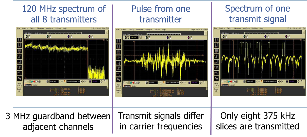
Figure 6. Transmitter outputs.

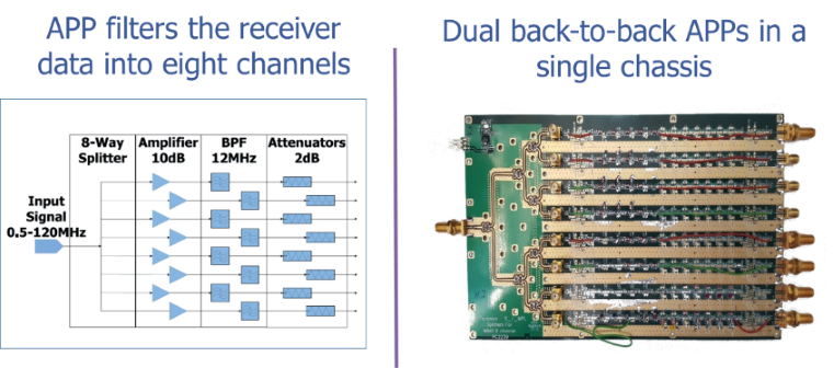
A custom-built analog pre-processor (APP) splits the 120 MHz baseband analog signal from the waveform generator in 8 channels (Figure 7). The 9 dB attenuation due to 8-channel splitter is compensated with the use of 10 dB amplifier for each channel. The signal corresponding to each transmitter is then filtered using BPFs with 12 MHz passband. Only the first transmitter channel uses a low-pass filter as it is difficult to practically realize a bandpass filter with a passband close to zero. The first five channels use Chebyshev filter design and the rest are elliptic filters, all with a passband ripple of 0.1 dB. Since subsampling raises the out-of-band noise, all of these front-end filters are designed to provide approximately 30 dB stopband attenuation. The imbalance in gain and spectral distortion are corrected by placing tunable equalizers at the end of APP chain.

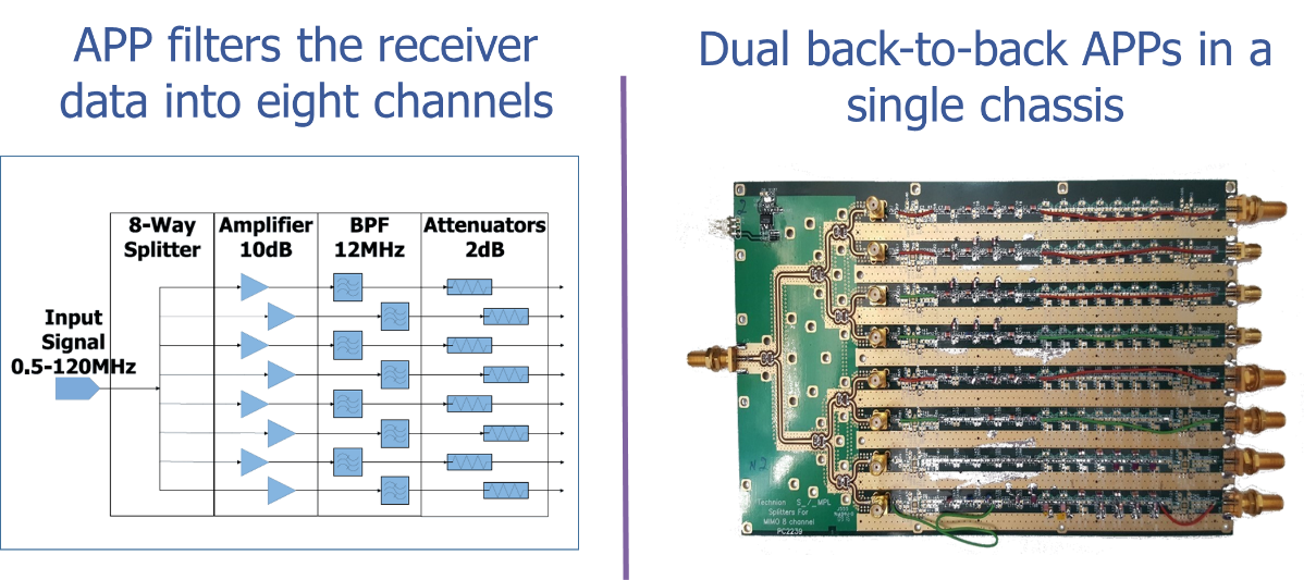
Figure 7. Analog pre-processor card. BPFs have ~30 dB stopband attenuation to mitigate subsampling noise

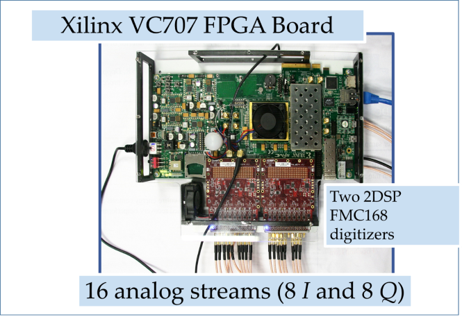
The channelized I/Q analog signals are then digitized using low-rate 16-bit ADCs in a digital receiver card (Figure 8). A digital receiver is realized using a single Xilinx VC707 evaluation board with two eight-channel 4DSP FMC168 digitizer daughter cards, one each for I and Q signals. The digital receiver output is transferred over LAN to a radar display (Figure 9).

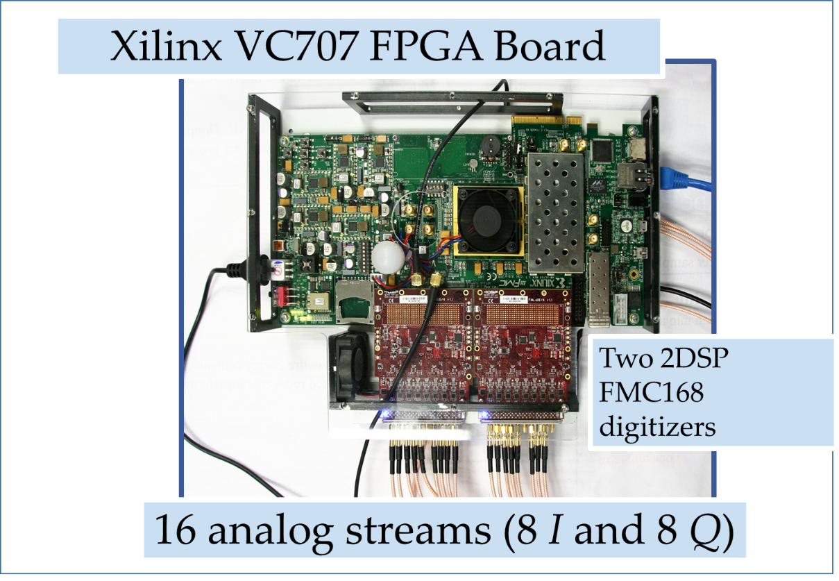
Figure 8. Digital receiver employs two 16-bit eight-channel digitizers for I and Q streams.

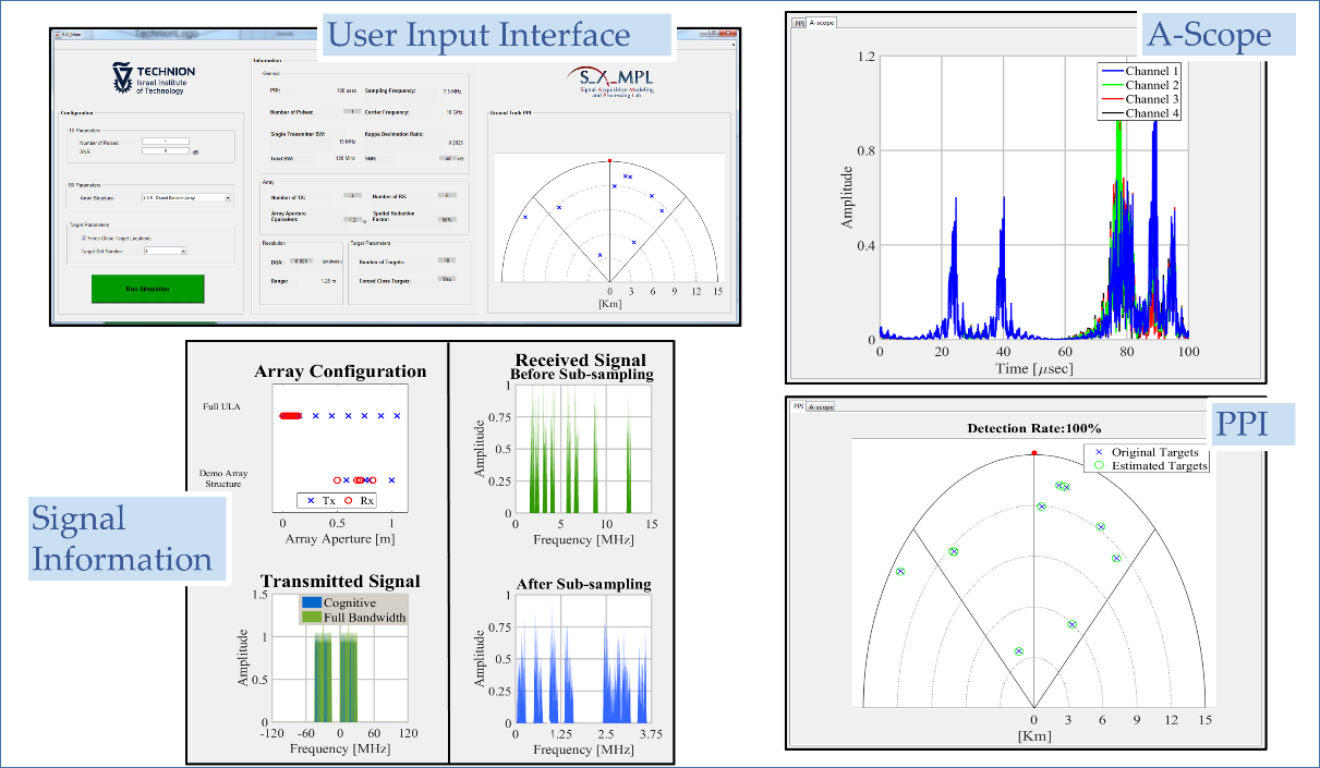
Figure 9. Radar display for sub-Nyquist cognitive MIMO.

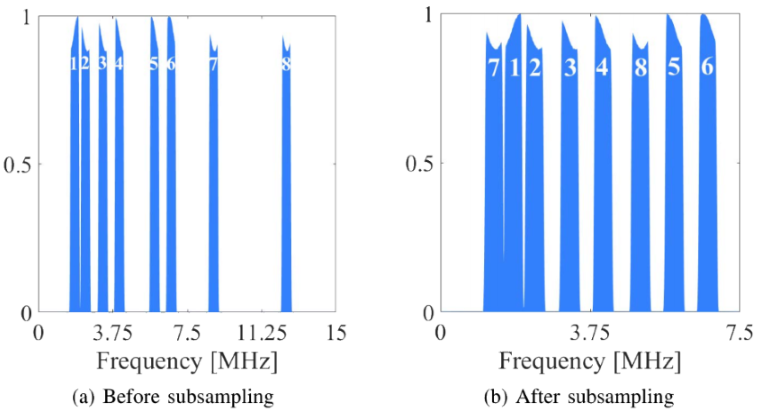
As shown in the following Figure 10a, the cognitive radar signal occupies only certain subbands in a 15 MHz band. Here, the sliced transmit signal has eight subbands each of width 375 kHz with the frequency range of 1.63-2, 2.16-2.53, 3.05-3.42, 3.88-4.25, 5.66-6.03, 6.51-6.88, 8.64-9.01 and 12.32-12.69 MHz before subsampling. The resulting coherence for this selection of Fourier coefficients is 0.42. The total signal bandwidth is 0.375 × 8 = 3 MHz. This signal is subsampled at 7.5 MHz and, as shown in Figure 10b, there is no aliasing between different subbands. A non-cognitive signal would have occupied entire 15 MHz spectrum requiring a Nyquist sampling rate of 30 MHz.

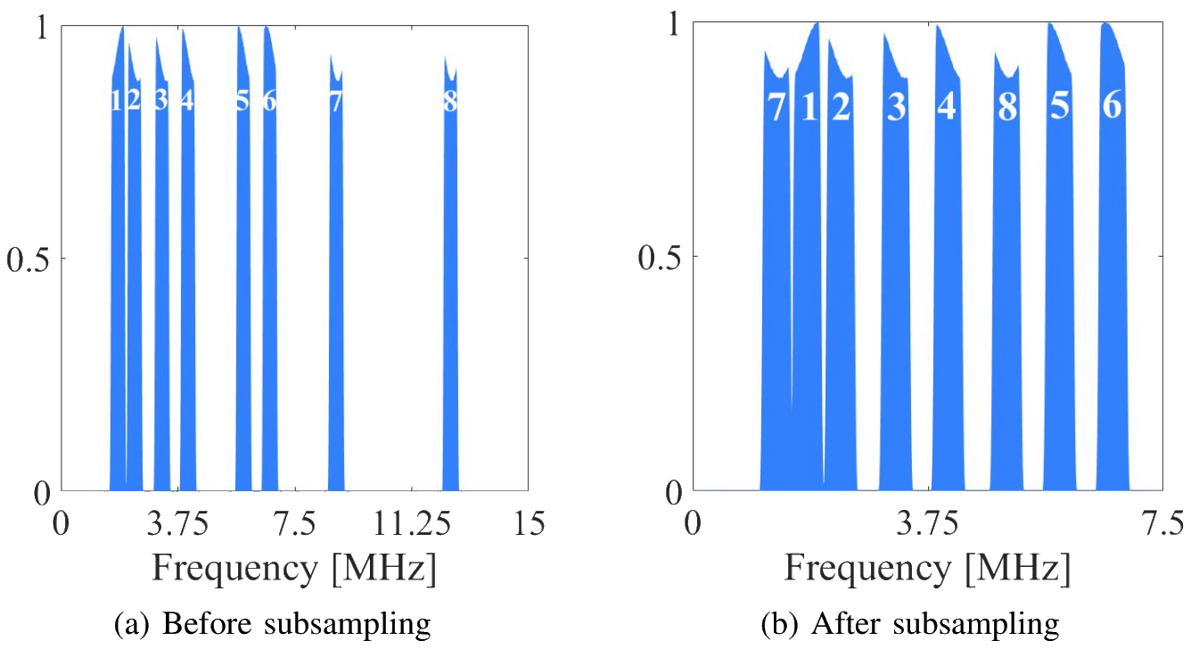
Figure 10. The normalized one-sided spectrum of one channel of a given receiver (a) before and (b) after subsampling with a 7.5 MHz ADC. Each of the subbands span 375 kHz and is marked with a numeric label. In a non-cognitive processing, the signal occupies the entire 15 MHz spectrum before sampling.

Therefore, use of cognitive transmission enables spectral sampling reduction by a factor of 4 (= 30 MHz/7.5 MHz) for each channel. Depending on whether the guard-bands of non-cognitive transmission are included in the computation or not, the effective signal bandwidth is reduced by a factor of 5 (= 15 MHz/3 MHz) or 4 (= 12 MHz/3 MHz) respectively for each channel. Mode 3 has 50% spatial sampling reduction when compared with Mode 1 or 2. If we account for both spatial and spectral sampling reduction in Mode 3, then we use a total one-eighth of the Nyquist sampling rate and one-tenth of the Nyquist signal bandwidth (guard-bands included). The sampling rate reduction is, therefore, seven-eighth or 87.5% in Mode 3. The receiver processes 80 and 20 channels in 8x10 and 4x5 arrays, respectively. So, the hardware resources are reduced by 75% in Mode 3.

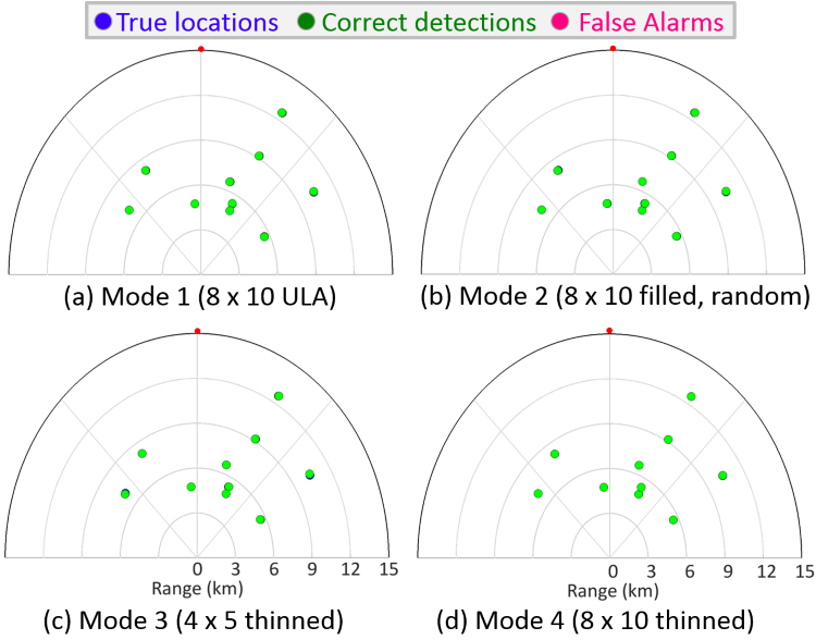
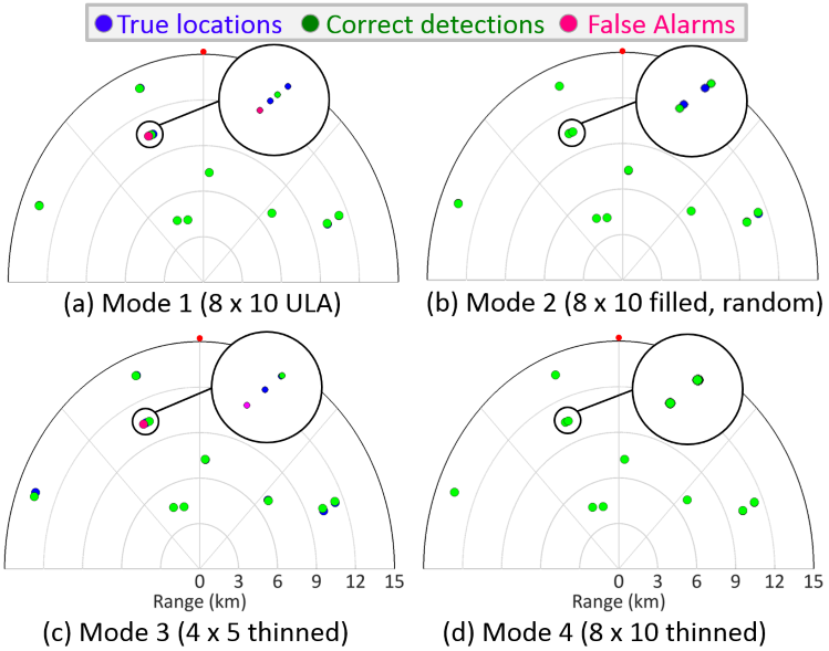
We evaluated the performance of all the modes through hardware simulations. Only one pulse was transmitted in all experiments and all modes were evaluated against the identical target scenarios. We injected the received signal corresponding to the echoes from 10 targets, placed at arbitrary range and azimuths, in the transmit waveform generator. In the first experiment, when the minimum angular spacing (in terms of the sine of DoA) between any two targets was approximately 0.025, the recovery performance of the thinned 4×5 array in Mode 3 was not worse than Modes 1 and 2 until the noise was dramatically increased. Figure 11 shows the detection performance of all the modes for this experiment when the signal SNR = −5 dB; the injected noise is complex white Gaussian. Here, a successful detection (green circle) occurs when the estimated target is within two range cells and one DoA bin of the ground truth (blue circle); otherwise, the estimated target is labeled as a false alarm (magenta circle). In case of high SNR or absence of noise, our criterion for successful detection is sensu stricto, i.e. the estimated target must lie at the exact location of the ground truth for a successful detection.

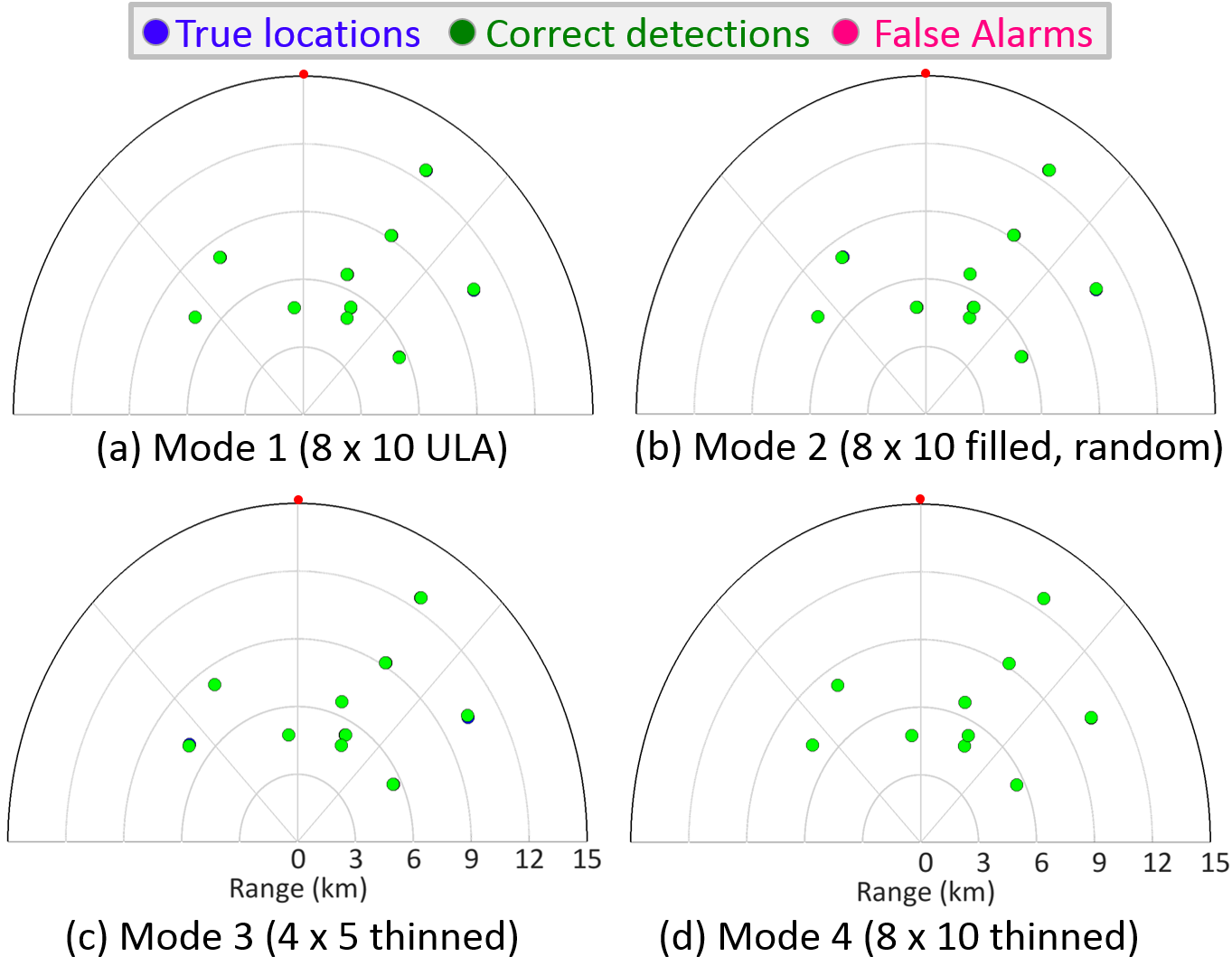
Figure 11. Plan Position Indicator (PPI) display of results for Mode 1 and 3. The origin is the location of the radar. The red dot indicates the north direction relative to the radar. Positive (negative) distances along the horizontal axis correspond to the east (west) of the radar. Similarly, positive (negative) distances along the vertical axis correspond to the north (south) of the radar. The estimated targets are plotted over the ground truth.

In the second experiment, the minimum angular spacing between the two targets was reduced to 0.02, and the SNR of the injected signal remained at −5 dB. Since the angular resolution of Mode 4 is better than the other three modes (see Table I), all the targets are detected successfully in Mode 4. Mode 1 and 3 showed a false alarm as seen in the inset plots of Figure 12. The Mode 2 also shows successful recovery in the broad sense of our detection criterion. The strict sense location error in Mode 2 is clearly larger than that in Mode 4. However, relatively better performance of Mode 2 over Modes 1 and 3 is not entirely fortuitous here. Figure 2 shows that both Tx and Rx array elements in Mode 2 are distributed such that its virtual array is wider than Modes 1 and 3. Thus, the effective angular resolution for Mode 2 could be better than 1 and 3, but still worse than 4.

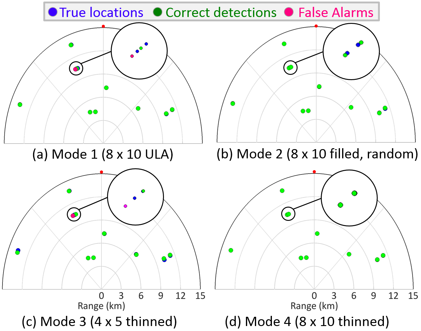
Figure 12. As in Fig. 11, but for a closely-spaced target scenario. The inset plots show the selected region in each PPI display at a magnified scale.

Software & Hardware:   SoftwareHardwareDemo movies