Algorithm

                 In this section we’ll explain how does the project work. It’ll be short explanation, the full one You can find in project book.

Algorithm

Home

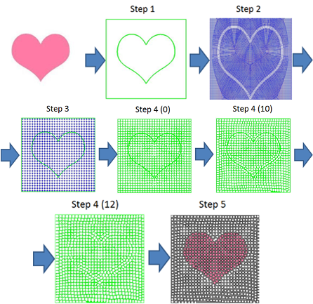
Main Steps

1. Creating an edge image

2. Creating a direction field based on the edge image

3. Choosing a list of points to begin with

4. Building CVD with respect to the direction field

Tile variations : color, size, aspect ratio. All those steps are fully detailed later in the document. A shortly visual description is added in the following section:

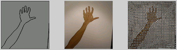
Creating edge image

In order to create a good edge image that contains all the majority edges but not all of them, we built a GUI that gives the user both automatic and manual options.

Automatic option

· The user can choose between varied edge algorithms and their parameters.

Manual option

· The user can delete or add curves to the image by using the mouse or touchpad.

 

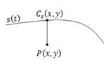
Creating direction field:

Definitions:

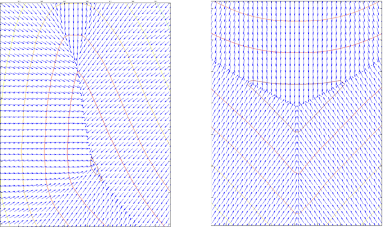
Algorithm

1. Creating the surface whose explicit form is

2. Evaluate the gradient

3. For a collection S of curves, let d s ( x; y ) be the distance to the nearest curve in S . For each curve s in S, the surface whose explicit form is z = d s S ( x; y ) resembles a long, curved mountain (s is the mountain ridge). If we 1) draw such a mountain for every curved edge feature in the image 2) numerically evaluate the gradient r z at each pixel, we obtain an image-precision form of z , the direction field we need.

 

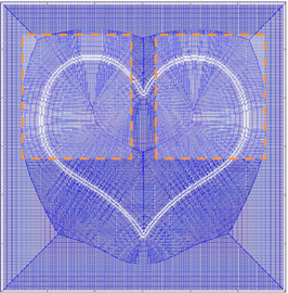
Examples:

 

 

Zoom in:

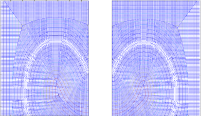
More zoom in:

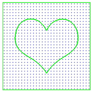
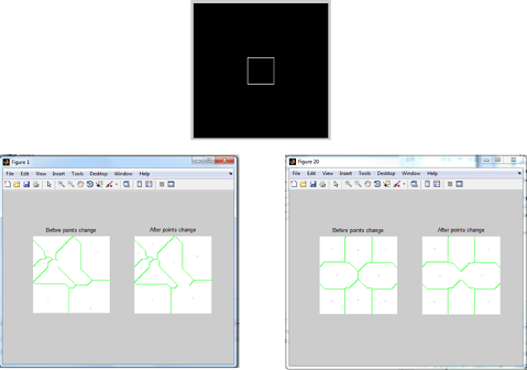
Choosing a list of points:

As a start list of points, we define the length between each two points and create a list of uniform points that cover all the image size. If a point is falling on the edge of the image, we take care that these points will move to another place so it won't fall on the edge. In the CVD iterations, these points will move until we achieve a perfect covering.

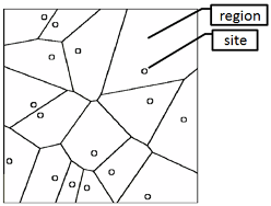
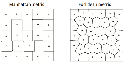
Build CVD:

Introduction

A Voronoi diagram is defined by collection of N sites and divides the plane into N regions such that all points within a region are closest to its associated site.

CVD is Voronoi diagram with the additional property that each site is located at the mass center of its region.

The distance can be measured by the Euclidean metric

or by Manhattan metric

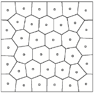
Algorithm:

1. S ß list of points on the image

2. Repeat until converged:

3. Repeat until the image is covered:

4. For each p in S, place a little square oriented along    .

5. Enlarge the squares equally.

6. If there is an overlapping  between the squares it’s a part of the Voronoi diagram

7. Compute the centroid of each Voronoi region.

Move each p to the centroid of its Voronoi region

Examples:

The following examples show the result of the algorithm after 20 iterations with a metric that was defined by a rectangle shown in the head of each example.

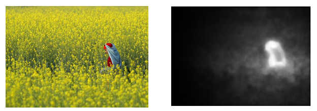
Using Saliency Project

In order to use more than one tile size especially in specific areas in the picture, we are using the Saliency Project.

The Saliency project extracts from an image the major details and gives them high weight while the background of the image, for example, gets low weight.

Example:

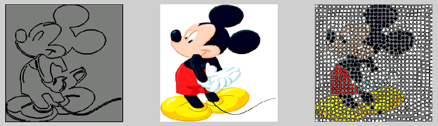
Algorithm

1. Creating mask

a. Creating saliency image

b. Creating a binary image by using low and high thresholds

c. Enlarging the edge of the original image.

d. Subtract the enlarged edge from the binary image.

e. Getting list of points on the image.

f. Using the Mosaic creator with the list of points we got.

Putting tiles with the appropriate size in the appropriate place.

All the procedure of the algorithm is described visually in the next figure:

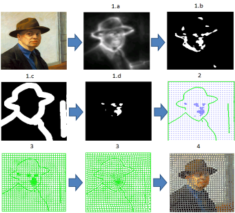
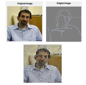
Results