
The Algorithm (please read notes first)
Initialization
Preparing Images
We implemented active contour image segmentation based on Bhattacharyya with Optical Flow.
Two models has been implemented. The main model is based on two-dimensional features vector, the second one is based on one-dimensional features vector.
Features vector determines the way to represent each image's pixel.
In the two-dimensional features vector model, we load two images from disk to Matlab, then we calculate optical flow (using [1]). As a result we get a new matrix that contains in each cell a two dimensional vector representing motion. We call this matrix features image, denoted by J(x).
In the one-dimensional features vector model that we created for learning purposes preceding our main model, after loading the image from disk we apply on it a standard Matlab function for converting it to gray-scale level. The resulting features image is a matrix that contains in each cell one dimensional vector representing gray-scale level of 8-bit resolution.
Another possible way to accomplish our task is to choose wisely the features
vector to contain both intensity and velocity. Such as
![]() while changing probability function accordingly.
while changing probability function accordingly.
![]() will be calculated using any Optical Flow method. But the additional
information from
will be calculated using any Optical Flow method. But the additional
information from
![]() might cause a better results and a bad results as well. Unfortunately,
we didn't had the time to try this.
might cause a better results and a bad results as well. Unfortunately,
we didn't had the time to try this.
The following table offers a brief overview of the steps mentioned above.
| 2d features vector (motion) | 1d features vector (gray-scale) |
|
|
Illustrations
Optical Flow*
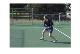 Frame 1 |
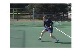 Frame 2 |
After applying Large Displacement Optical Flow algorithm, we get one matrix that contains in each cell two-dimensional vector. For the purpose of our explanation, we split the matrix to represent two velocities, one in the direction of x-axis and the second of y-axis. In other words, we split the two-dimensional vector in order to see things more clear.
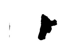 Velocity Over X-axis J(:,:,1) |
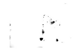 Velocity Over Y-axis J(:,:,2) |
Gray-scale convertion **
 Rabbit Color Image |
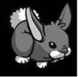 Rabbit Converted Image J(:,:) |
Features Vector Precision
The precision that is used in our project is 8-bit. It’s faster than 32-bit precision and gives good results compared to higher precision calculations.
In the two-dimensional features vector model, J(x) is created using Large Displacement Optical Flow which return features of double precision. As we mentioned above, double precision contain a great details and can give us even a better results! But it is heavy on calculations. Therefore, we decrease the resolution from 32-bit to 8-bit.
In the one-dimensional the features vector contains 8-bit precision as a result of applying the standard Matlab unsigned 8-bits conversion function. Therefore, no conversion needed.
Preparing Variables and Parameters
Before getting into the main loop, variables and parameters should be initialized. They will determine a lot of aspects of the main algorithm loop, such as the speed of the diffusion and number of iterations required and etc.
Two important variables are: the Kernel and the Level Set.
The Kernel
The probabilities densities in our project are estimated using the simple Gaussian distribution as a smoothing kernel. Using Gaussian one-dimensional kernel enables us to perform fast separable convolutions.
What is seperable filter anyway?
"A two-dimensional filter kernel is separable if it can be expressed as the outer product of two vectors." [2]
What is the point behind seperable convolutions?
It's simply faster. Filtering an M-by-N image with a P-by-Q filter kernel requires roughly MNPQ multiplies and adds (adds usually has a neglictable effect on time complexity) . If the kernel is separable, you can filter in two steps. The first step requires about MNP multiplies and adds. The second requires about MNQ multiplies and adds, for a total of MN(P + Q). [2]
The computational advantage of separable convolution versus nonseparable convolution is therefore:
![]()
Back to our project, Gaussian kernel is seperable.
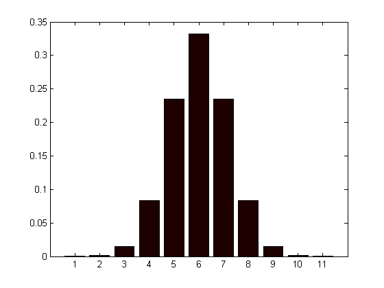 one-dimensional Gaussian (h) displayed using bar() function |
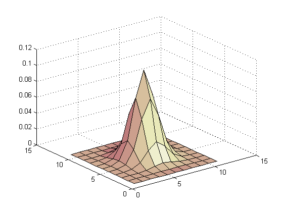 two-dimensional Gaussian (h*h') displayed using surfl() function |
In our case, for a 11-by-11 Gaussian kernel, we gain a speed-up of 5.5.
![]() To
make use of this speed-up, all that should be done is to perform sequent
convolution with h, without using h*h' directly. Note
that this advantage is only on two-dimensional convolution.
To
make use of this speed-up, all that should be done is to perform sequent
convolution with h, without using h*h' directly. Note
that this advantage is only on two-dimensional convolution.
Level-Set Function
The Level-Set function is the most important one. All the dynamic calculations are performed on it. Furthermore, the contour is derived from the Level-Set function where the value is 0.
At initialization, the Level-Set is set according to the user's choice of the contour. The initial contour is formulated using the simple ellipse formula after the user chooses the area.
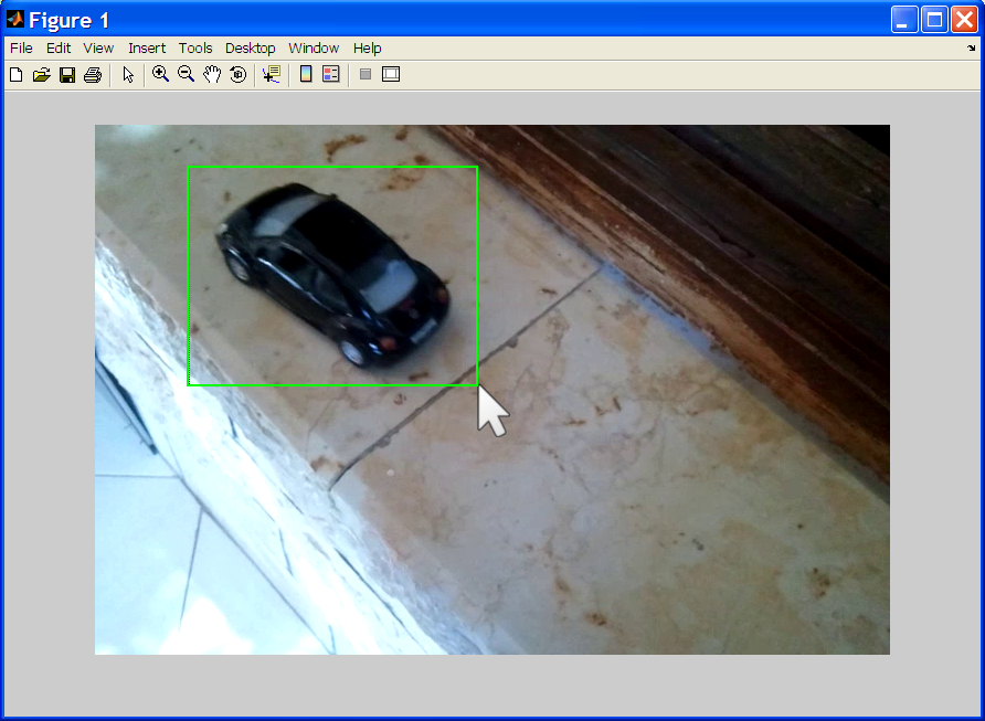
Afterwards, the Level-Set function φ(x,y) is formulated in two steps. First, an auxillary surface I(x,y) is created. I(x,y) will contain a surface of only two values, 0 and 1. 1 inside the edges of the ellipse whose center is the chosen area's center, and 0 outside. Then φ(x,y) is created using the information in I(x,y) with the help of bwdist standard Matlab function.
bwdist(BW) computes the Euclidean distance transform of the
binary image BW. For each pixel in BW, the distance transform assigns a number that is the distance between that pixel and the nearest nonzero pixel of BW. [3]
φ(x,y)=double((I==0).*(bwdist(I==1)-0.5)-(I==1).*(bwdist(I==0)-0.5));
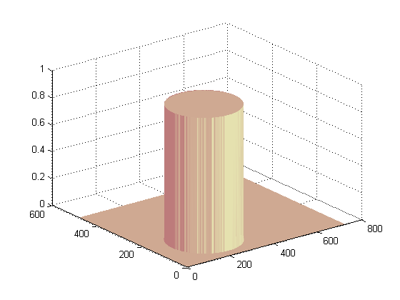
auxillary function I(x,y) surface plot
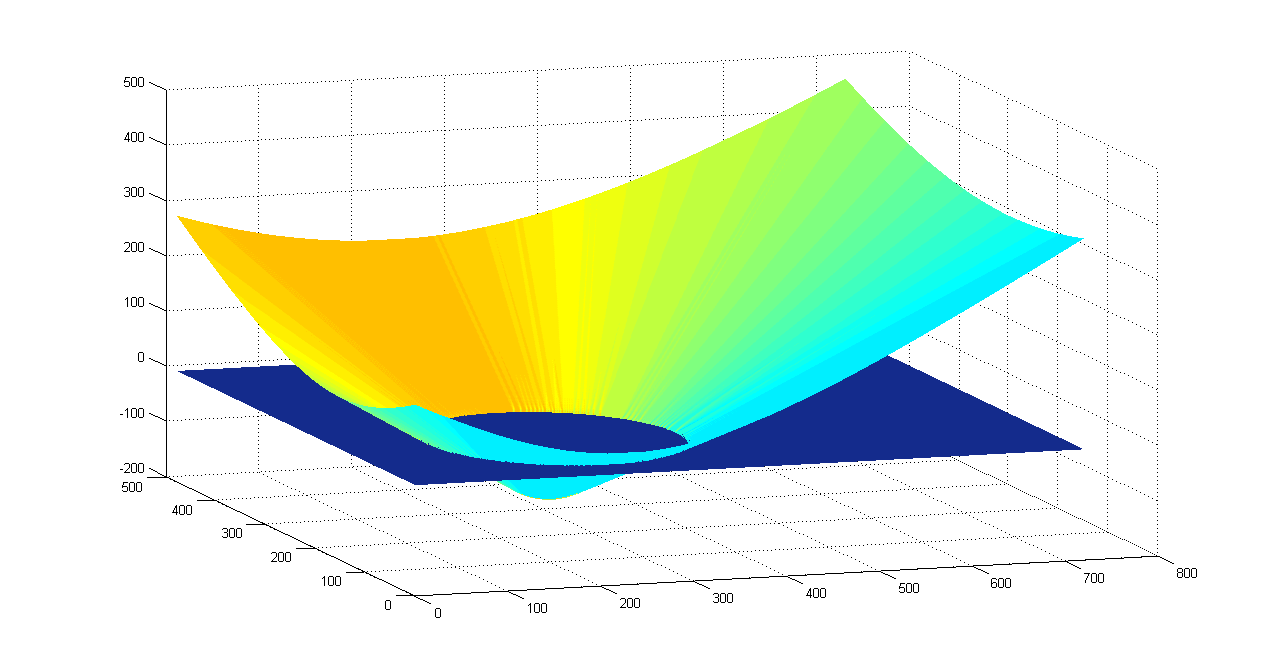
level-set function φ(x,y) surface plot
That's it all regarding initialization that we are about to explain. If you need to know more please have a look on the code, it's self explanatory.
Main Algorithm Loop
The algorithm works in iterations. In each iteration, calculations is being made to move the contour towards the real object edges. This is achieved in following steps:
-
Calculating the gradient flow which is denoted by V(x,y)
-
Changing the Level-Set function φ(x,y) accordingly.
-
Updating the features probabilities functions inside and outside. Denoted by Pin(x,y), Pout(x,y), respectively.
Each of the steps above is explained in details. It’s obvious that the general outline of the algorithm shows how adjustable it is. This is very important when it comes to fitting the algorithm to different fields, or optimizing it for a certain usage.
The loop will stop when the change in the gradient flow is smaller than a fixed threshold. Because when this occurs, it indicates that the deformable contour is very close to the real object edges.
Gradient Flow
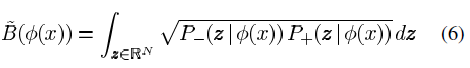
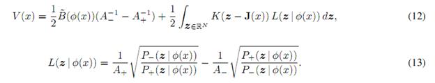
In order to minimize the Bhattacharyya coefficient, its first order variation should be computed.
The Bhattacharyya coefficient is defined as:
While the feature probabilities are defined as:
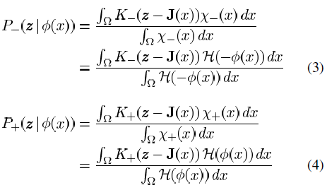
As we mentioned above, the Kernel function K(x) that we used in this project is Gaussian density distribution.
Heaviside function H(x) is used to distinguish between points inside and outside, based on the Level-Set function φ(x,y).
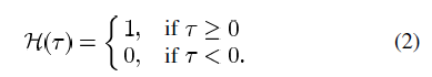
Remember that the Level-Set function φ(x,y) can represent 3 important sets of points in the following way:
-
The contour is where the Level-Set values equals 0.
-
The points inside the contour are where values is smaller than 0.
-
The points outside the contour are where values are greater than 0.
The first order variation V(x,y) is computed in the following way:
Level-Set
After computing V(x,y), reevaluating φ(x,y) is easy. What is achieved during this phase is moving the contour in the direction of the real object edges.
The idea behind this is that the first variation of the Energy function which in our case is the Bhattacharyya, tells us exactly where we should move to minimize the energy function, thus minimizing distance between probability distributions. [see Overview].
![]()
The speed of diffusion is denoted by c which is set in the initialization phase.
More filters and methods can be applied on φ(x,y) to have better results.
Probabilities
Features probabilities densities could be computed easily like we did in the initialization. We should be aware of the downside of this convenience. It is the fact that this process is heavy when it starts all over again after each of the iterations. Luckily, the way that those probabilities densities are defined allows us to optimize this calculation in the following way:
![]()
![]()
While
![]() represents the set of points which were originally involved, and
represents the set of points which were originally involved, and
![]() represents the “excluded” points. In other words,
represents the “excluded” points. In other words,
![]() can be updated using (28).
can be updated using (28).
The above formula (28) is optimal because it takes into account only the points who changes as a result of the contour deformation.
Notes
- The one-dimensional model (gray-scale) is not the main model, but it's mentioned to allow one, through the comparison, to understand how motion features are utilized.
- Number of symbols writen in function's range do not is precisely reflect the range dimention. e.g. f(x) range might be two dimensional.
- Function's range symbols do not is precisely define a certain space. e.g. f(x) and g(x) ranges might be different even if range's symbol is x.
- Code snippets are avoided as much as possible to keep explanation neat and tidy.
- Matlab code files are well documented. [see Files]
References:
[1] T. Brox, J. Malik. "Large displacement optical flow: descriptor matching in variational motion estimation" 2011
[2] Separable Convolution. Matlab Central. [>]
[3] bwdist documentation. MathWorks. [>]