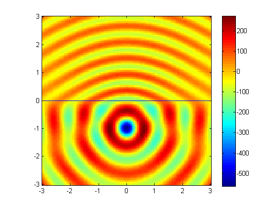
Calculation of the field of a line-source in front of dielectric half-space.
This example shows how to use the ND-SDP method.
Contents
Set-up some global variablesclear
initialize_globals
Set-up parameterspermittivityLowerRegion = 1;
permittivityUpperRegion = 3;
componentString = 'Ez';
Source parameterslambda = 1;
Source.lambda = lambda;
Source.polarizationString = 'TM';
Source.x = 0; Source.y = -lambda;
Grid points at which the field is to be evaluatednX = 100; nY = nX;
r = lambda*3;
x = linspace(-r, r, nX);
y = linspace(-r, r, nY);
[EvalAt.x, EvalAt.y] = meshgrid(x,y);
Set optionsOptions.quasistaticRule = 'discretization';
Options.useAdaptive = false;
Options.nPoints = 20;
Options.tol = 1e-3;
Options.maxPoints = 2^10;
Calculate fieldtic
field = ndsdp(EvalAt, Source, permittivityLowerRegion, permittivityUpperRegion, componentString, Options);
toc
Elapsed time is 3.651567 seconds.
Show the resultclf
imagesc(x/lambda, y/lambda, real(field));
set(gca, 'ydir', 'normal');
axis image
colorbar
line([min(x/lambda), max(x/lambda)], [0 0])
 |